Setting Up a Student Sheet for Success

 Setting up a sheet well for someone else to use, whether that sheet is for students or teachers, can make or break its success. This post will focus on conventions that I use to make my sheets easier for users. That being said, just as curb cutouts started as a way to make sidewalks easier for differently abled people, they actually help everyone. These conventions will help everyone who uses the sheet, including you!

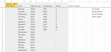
Often organization elements are left with header color and alternating rows. This isn’t surprising because traditional spreadsheets are table based - basically accounting tools. This is leaving a lot of the table, especially if you are working with folks who have limited spreadsheet experience. Take the two examples below of the same gradebook template. This template is meant to be used by middle school students. 

Example 1

Example 2

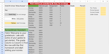
Here the goal is to teach students some introductory spreadsheet calculation skills. I would argue that the first example is opaque and even anxiety provoking. The second example uses color to focus attention on important elements, includes a Key to give the user context, and even uses a “Spreadsheet Assistant.” This handy box contains an IF/THEN/ELSE statement that changes as the user begins to build the sheet, giving the student a sequence of steps. Doing it this way takes more set up time, but it will save you and your students so much frustration on the other side. This tutorial will briefly talk about using color, making an IF/THEN assistant, locking elements so that users don’t change the wrong thing, creating a data feed, and will introduce a discussion about distribution.

Lets Talk Color and Merging

---

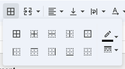
We are visual creatures. I love a good table but only when I need to organize lots of data. All those columns and rows can be visual noise if your project is more of an interface. Simply put, making the cell and border colors the same creates a cleaner visual experience. The lines can disappear where they aren’t needed. Cells can be merged to create specific areas with a larger text box, as with the spreadsheet assistant in the example. The border tool can add an underline, bring all the rows back, or simply create a box around an area, like in the Sheet Key example above.

The IF/THEN Assistant

---

IF/THEN statements are incredibly powerful and can be very complex. These statements can look for matches, include OR statements, employ mathematical formulas, and so much more. The statement that creates the Spreadsheet Assistant can be quite simple. First, consider the steps that you would like your students to follow. Make a chart on your variables tab with a step number column and an instruction column and start to brainstorm a lesson sequence. You can type these directions directly into the IF/THEN statement but I find using a chart easier to plan and edit later.

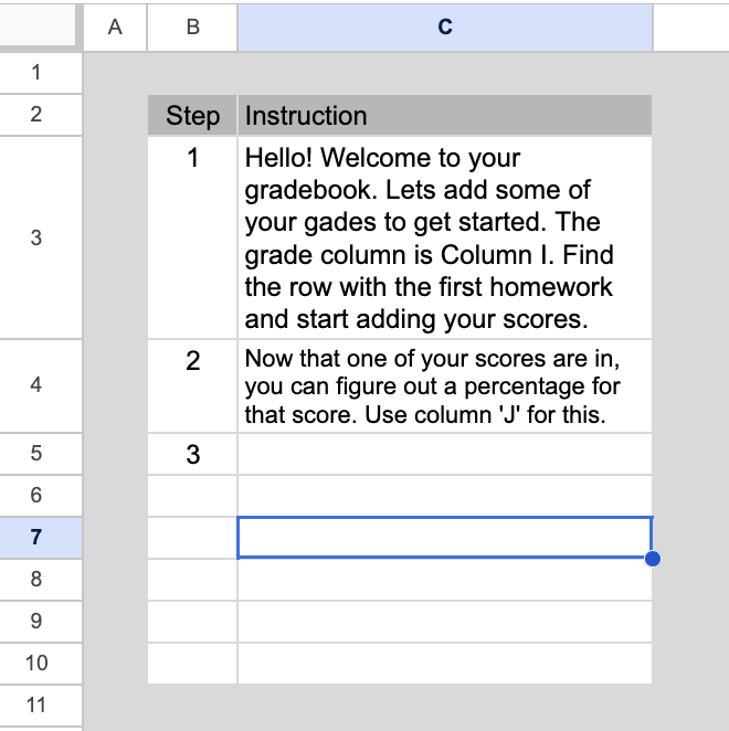
Once your instructions are laid out, the statement is easy to compose. The syntax of an IF/THEN/ELSE statement is:

IF(logical_expression, value_if_true, else)

My first instruction looks to see if any scores have been added to the score column (I). I’ll do this by using a SUM function for the entire range, just in case a student adds a score next to a date further down the list. If the sum is less than 1, then the assistant box will contain instructions for step one on the variables sheet (Variables!C3):

=IF( SUM(I3:I)<1,Variables!C3,

My ELSE statement will be the condition for the next instruction. In this case, whether or not any percentages have been added to column J. If not, the second instruction will load (Variables!C4):

=IF( SUM(I3:I)<1,Variables!C3, IF( SUM(J3:J)<1, Variables!C4,))

And so on! The nested IF/THEN statement can provide steps for the entire project!

Locking Elements

---

We will use a tool called Autocrat to distribute copies of the gradebook template to each student in your classes. When we do this, you will retain ownership of each sheet and you can control the level of sharing that you students possess. In this case, each student will be an editor. Because of this, you can lock particular sheets, ranges, even specific cells, that the students won’t be able to edit. Some careful consideration should be made into what cells are locked. With our gradebook, we can lock everything in the columns between A and H. Those will be teacher columns. We also want to protect the Variables sheet, at a minimum. When the sheet is distributed to your class, these protections will be maintained. Google provides a nice guide to protecting sheets and ranges here.

Creating a Data Feed

---

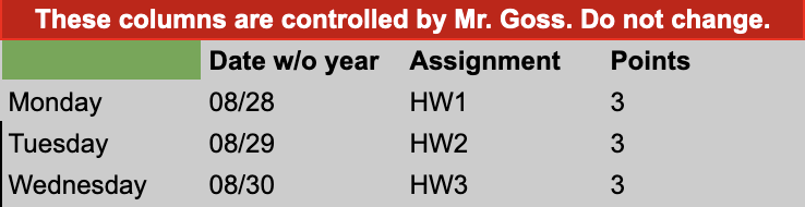
The gradebook has to be useful and easy to use. One way to do this is by feeding in data and reducing the amount of text input for students. We are going to feed in the dates for the school year, the days of the week for those dates, the assignments and tests corresponding to the dates, and the maximum score possible for each. All of this information is fed from a master sheet. The master sheet is a lesson unto itself.  This automatically creates a list of dates between two given variables, making it easy to reuse each year. You can read about how to build it here. The data is instantly sent to each student’s sheet whenever the teacher adds an assignment to the master and setting it up is easy. We will be using a function name IMPORTRANGE which allows you to pull data from a different sheet. The source sheet must be shared with the user in order for the import to work. None of this data is sensitive so it will be easy to share the source sheet as read only. We can turn off notifications, too, so that it doesn’t send an email when shared. The syntax for import range is simple:

=IMPORTRANGE(spreadsheet_url, range_string)

The first condition is the url of the source sheet, surrounded by quotes. The second condition is the location of the data range in the sheet, also surrounded by quotes:

=IMPORTRANGE("https://docs.google.com/spreadsheets/d/1UBVC6dwwH1UGnR91do-bu4RV8xM9CsTh_2oJPw-Vhdg/edit#gid=1017551313", "Scheduler!C3:H294")

There will be no data when the student opens the gradebook for the first time. The student must give permission to the connection. I usually create cues to help this process. In our example sheet I write “Click B1 & then “Allow Access” and point to cell B1 which I have made green. When a student does this (even though it is protected and the student can’t change the function) a button will appear requesting him or her to “Allow Access.” The data will feed in once access is granted!

Distribution

---

You cannot distribute your sheet to your class until it is completely ready. We will have a separate tutorial later about using the Autocrat extension for this purpose. In the meantime, you can set up a spreadsheet with your class rosters. This sheet will need a row for each student. The data should include the student’s first and last name, and email address at a minimum. Additional useful information could include period number, parent email (you could share it with parent as a read only doc,) learning resource teacher or case manager email, and more. When autocrat is run you will have a handy link to each student’s gradebook added to each row.

Next time we will work with an autocrat and go into the details regarding document distribution.

Extension activity:

Create a sheet in the gradebook with useful information for your students. Add a chart with the grading scale, create a reference for math symbols and share where to find them on the keyboard(^ is Shift + "6"), provide a list of tips for writing a math function (eg: All formulas must start with an equal sign)

Google Sheets Powered PO Generator

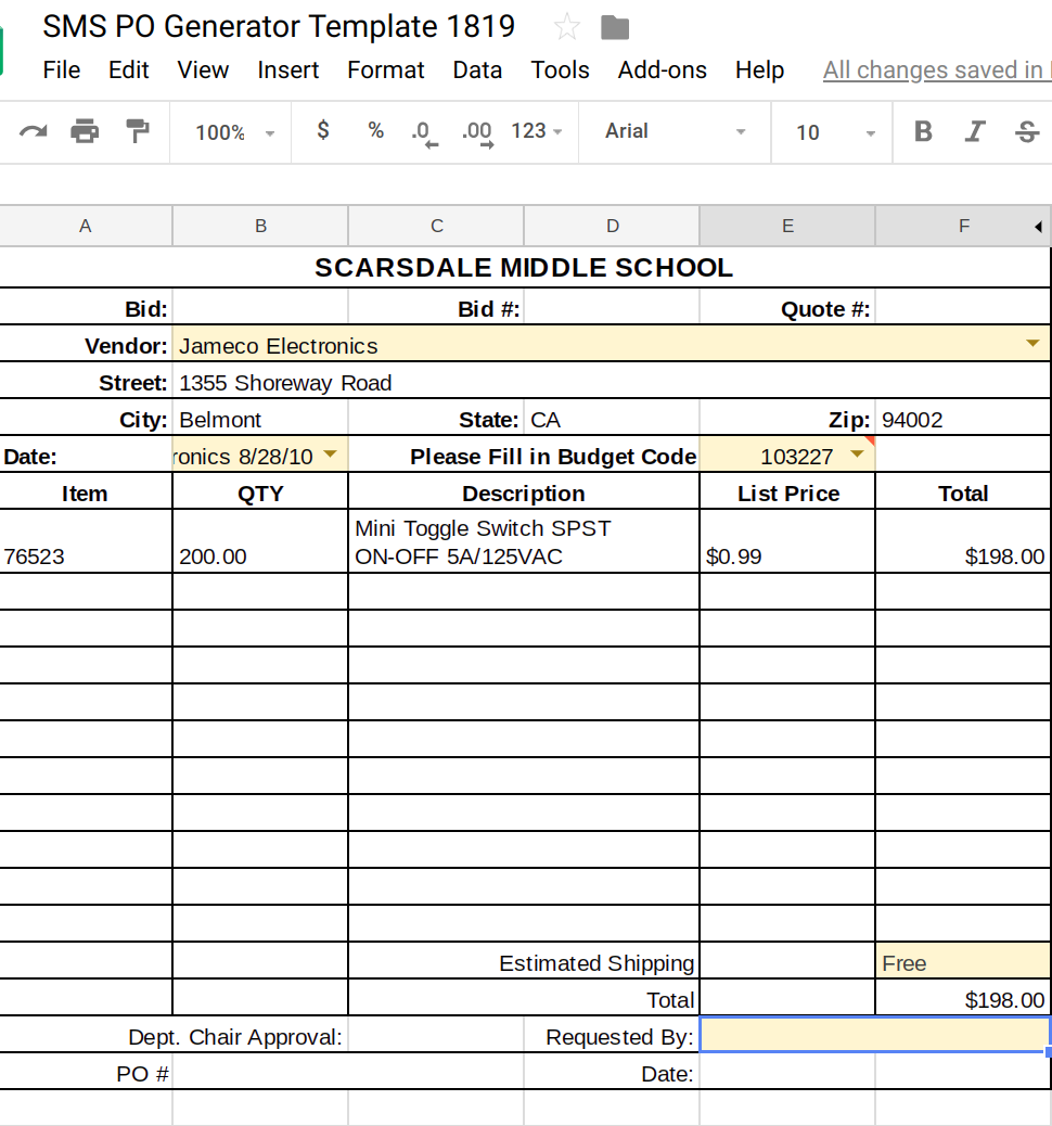
Writing purchase orders is one of the least favorite parts of my job. It’s often a repetitive and monotonous task that requires a deep dive into a file cabinet, a massive catalog, or both. I created this spreadsheet tool to make POs a little less onerous. This system keeps track of your orders, allows you to take notes, monitors your budget in different budget codes, and will actually generate the printed PO sheet! Make a copy if you would like to use the sheet. I hope you find this as useful as I do.

Setting up the sheet is easy. Just add your vendor information to the Vendor Tab. As a general rule, anything in the sheet with a yellow background can be edited. Anything with a grey or black should not be edited. These are controlled with functions. Adding vendor addresses is a one-time outlay of work. The address will auto-fill on the POs. I include my own information here, too, because there are certainly times when I purchase something from a vendor not on the bid list (Amazon, anyone?) and need to submit a PO with me as the vendor. You can add vendors as you need them, secure in the knowledge that the address will be ready the next time a PO is generated for that seller.

Also on the Vendor sheet is a budget code table. I have two budget codes as a technology teacher, one for supplies and another for equipment. In order to keep track of your codes, add the total amount you have to spend and the codes themselves in the appropriate columns (yellow only.) You’ll notice that the sheet automatically keeps track of the amount left in each budget code and the supplies code has a function that helps me keep track of per student expenditure.

The “Master Sheet” is where I fill out my orders (yellow cells only.) It's fairly self explanatory. One this thing I need to point out: the first two columns seem redundant but are not! The first column allows me to specify an order on a specific day, the second column is only the vendor name, linked to your vendor sheet. This second column controls the address information and is independent of the date. Both are necessary!

Once your order is recorded on the “Master Sheet” you can generate your PO. Now you have one place for all your PO records and you don’t have to worry about handwriting a PO form. Better yet, next year I have a clear record and can reorder easily. Open the PO Generator tab. You will notice four yellow cells, three with drop down boxes. Select your Vendor, which will populate all of the address fields. Then, select the date the PO was written, which is fed from the first column of the “Master Sheet.” Finally, select the budget code, write in the potential shipping cost, and add your name in the “Requested by:” field.

Your PO Is ready to print! This has made PO writing so much easier for me. I keep notes on my Master Sheet, such as when an order arrives, or if I was unhappy with the product. My record keeping is better and the process is a lot faster. This was designed using the Scarsdale PO form, so you may need to redesign the PO Generator layout. Let me know if you use this and if you’ve made it better!

Build a Commenting system With These 5 Spreadsheet Tips

Google elevates the humble spreadsheet by bundling in forms, multi-user capacity, and the inherent connectivity of the Internet. This combination gives Google Spreadsheet application authoring-like chops. This post is going to explore this idea by making a moderated comment system using a few spreadsheet tricks.

You might ask, “Why?” Well, this system uses some functions that I use a lot, so it's a handy vehicle to talk about them. That said, there are reasons why we've used this at Quaker Ridge. Some sites don’t have built in commenting features, especially sites built on education content management systems. Other platforms, like Google Sites, have comments, but they can’t be moderated. Systems like Disqus are popular and powerful, but give you little control over what is done with your data. This is gross in general, but it’s particularly foul in the K-12 edu space. Finally, it can be more communal than a blog post comment. We can create a meta comment feed that insulates young children from the “I don’t get any comments but my friend gets so many” problem. So here you go, 5 tips to make your own comment system!

Tip 1: Use Validation!

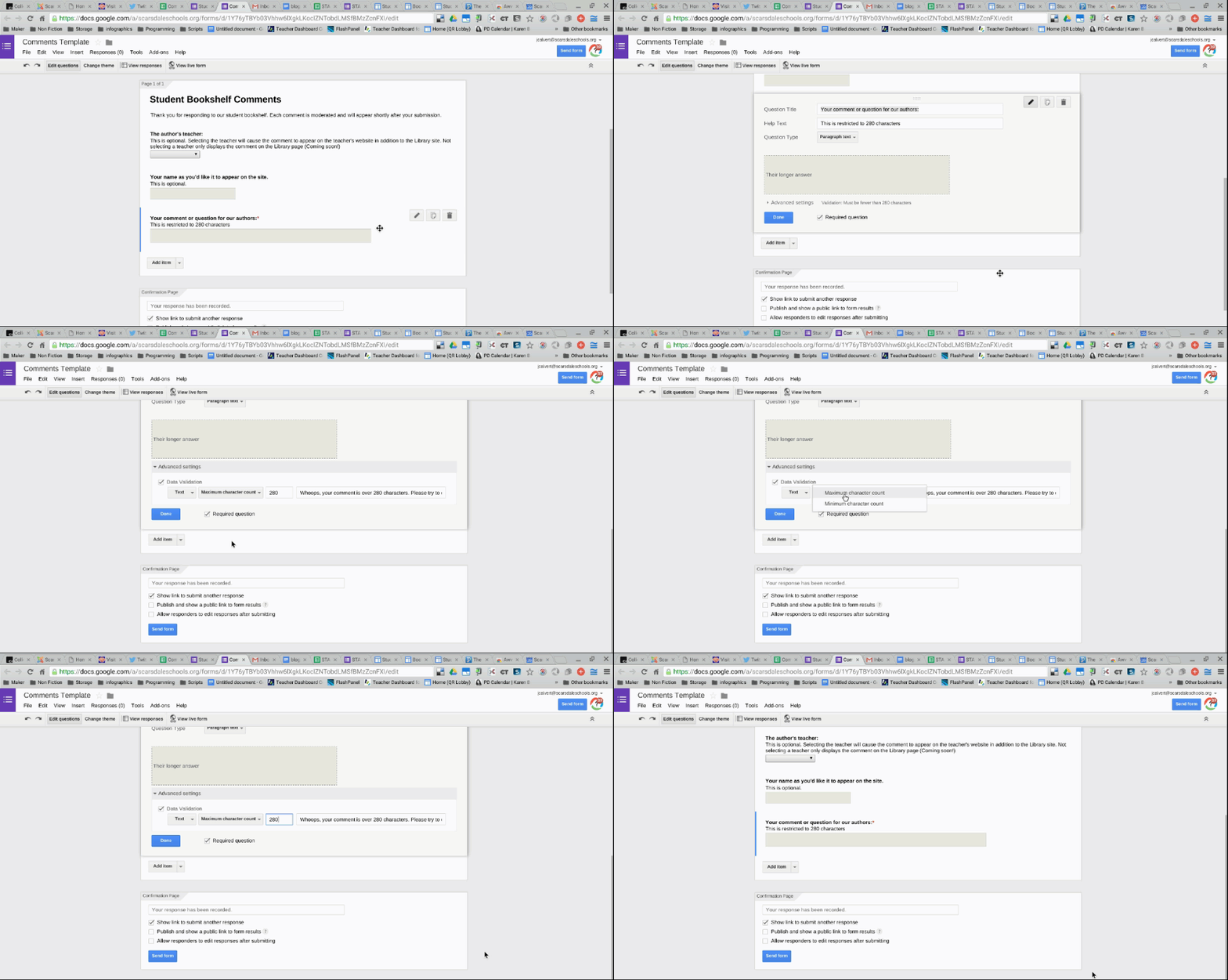
Every good comment system needs a form to submit. My comment form has three questions, a teacher name drop down so that the comments can be filtered by class. An optional text box so that the person commenting can leave a name if wanted. And a paragraph text box for the comment. This last item is validated (click the advanced settings under the question) to 280 characters. I figure that twice the length of a tweet is enough to ask a question or provide feedback, but adjust accordingly.

Tip 2:  Use a QUERY for Moderation

I use this trick often. You’ll also find it in the Twitter Exit Ticket and the Book Review form. A query will take data from one page and display it on another, based on criteria that you declare. This criteria could be a number rage, or specific values, and can use boolean operators such as “OR” and “AND.”  I simply add a “Moderation” column to the right of my form sheet. Then, I add a query to a new sheet that watches this column for a value of ‘yes.’

=QUERY(data!A1:E, "where E = 'yes'",1)

This sheet is what gets sorted by the comment page. Since I use one system for several teachers, I include the “AND” operator to also look for a specific teacher’s name.

=QUERY(data!A1:E, "where E = 'yes' AND B = 'Teacher 1'",1)

It’s useful to learn how to write a query, but until you do, just use Bjorn Behrendt’s very cool EZ Query add-on.

Tip 3: Reverse the Order of the Comments
When someone submits a Google Form, the last response shows up under the previous submissions. Typically, you want the opposite with comments, with most recent submission first. We can use a SORT function to change the order. Add another sheet and sort the approved comment range using the timestamp column (represented by the 1) as the sort by column.

=ArrayFormula(sort('Tip 2: Moderate'!A2:D, 1,false))

Tip 4: Join Columns With Linebreaks

A comment system will often include who made the comment and the date the comment was submitted. Unfortunately, these items are in different columns. We need to join these together and do it in an attractive way. Columns can simply be joined by using the “&” symbol. However, we also want the columns separated with carriage returns - otherwise it would look crowded. The character code for a return is “CHAR(10).” We’ll use two together to create a space between the name and the comment..

=ArrayFormula(sort((" By: ")&'Tip 2: Moderate'!C2:C&CHAR(10)&CHAR(10)&'Tip 2: Moderate'!D2:D&CHAR(10)&CHAR(10),'Tip 2: Moderate'!A2:A,false))

Tip 5: Test for Blank Rows

The last function joined all of the rows, whether or not there was a comment. This left hundreds of orphaned “By:’s” from all those empty rows. Since we only want the function to apply to rows with comments, we can use an “If( ISBLANK( ‘Column’),”  test. This combination will look at a column, 'Teacher 2 Approved Comments'!C2:C in our case, and check each row for blanks. If a blank row is found, then nothing is done ("".) However, if something is found in a row, we can execute the joining formula from earlier to construct the comment.

=ArrayFormula(sort(IF(ISBLANK('Tip 2: Moderate'!C2:C), " ", " By: ")&'Tip 2: Moderate'!C2:C&CHAR(10)&CHAR(10)&'Tip 2: Moderate'!D2:D&CHAR(10)&CHAR(10),1,false))

Ready for Publishing

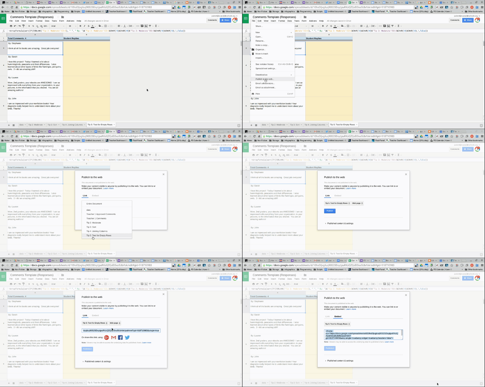
Now your comment page is ready to publish! Just click “File > Publish to the Web.” Select the comment page to publish and grab the Embed code. Then, paste that into any website that needs a moderated comment system! I’ll often set up the formMule add-on so that new comments will send an email to the teacher. Don’t forget to link to the form, too, and thanks for getting this far! Let me know in the comments if you have any questions.

How to Host Images on a Google Site for the Web

Images need a web address in order to be used in a system like Awesome Tables and this post explains one way to get it done. For our Online Book Review site, I used book covers that were hosted on Library Thing. But for builds that use your own images, like a student art gallery or an ebook shelf of student work, you need to host your own images. This is a niche post that I will reference when I write about making Awesome Tables sing with hosted images. If you are never going to use Awesome Tables or if you have a web server, well, you probably don’t need this post. Otherwise, read on!

Using a Google Site is an easy way to host files for free online. Google Sites in the wild have a 100MB limit, which translates into a lot of JPG files. Sites work a little differently Inside of an EDU domain. The whole domain is capped at a 10 GB quota.

I usually make one site to host my media files and create a page for each class or project. I share the site with the audience I need, whether it’s public, for the domain, or for a smaller group. Then, I add the jpg files with the “Add Files” attachment feature on the bottom of the page. This creates a weblink for each uploaded image. Right click on the JPG name and “Copy the link address,” but do not stop there!  This link won’t work for the public and you might not realize the problem. In an insidious twist - it will work for you, making you think everything is good, but others will see a broken image link.

To make the link valid, paste the URL where you need it to go (into a form or a piece of HTML for instance) and delete everything from the question mark, on. You will be left with a web link that can be used in an Awesome Table or any other HTML.

I hope this post comes in handy for you. If it does, let me know in the comments!

Embedding a Google Folder Into Your Teacher Site

Embedding a Google Folder is one of those things that is easy to do in a Google Site, but takes a little tinkering for other types of websites. My school system uses the SchoolWires CMS and my teachers routinely embed Google folders for newsletters, parent forms, and photos. This elegant solution makes updating your teacher site painless; just add the newsletter to the folder and it appears on your website. Lets look at how it’s done. If you are comfortable with creating and sharing Google folders, skip to Step 4.

Step 1

The first step is to create the folder in Google Drive and name it appropriately. Simply go to https://drive.google.com/ and click the red “Create” button on the left. Then, select “Folder.” Once you have named this new folder, it’s time to share it.

Step 2

Find the folder you’ve created in your Google Drive and double click to open. Once open, you will see breadcrumbs at the top telling you the path to this folder. This will look something like “My Drive > Your Folder Name.” Next to the name of your folder is a down-pointing arrow. Click this arrow to see the folder options menu. Then click "Share."

Step 3

The “share” window will appear. Find the small “Advanced” link on the bottom right and click this. The Advanced window will give you a few choices. The embedded folder will behave according to the sharing permissions that you set. From here you can share with specific people, share with a group, just your domain (if you are a GAfE school,) or make the folder public. We are going to make the folder public so that anyone visiting the website can see the contents. Click “Change” next to “Private - Only you can access.” Then, click the radio button next to “On- anyone with the link.” Press “Save,” then “Done.”

Step 4

Now that the folder is shared, you need copy the Folder ID. This is the string of letters and numbers at the end of the folder URL, after the last “/.” Select and copy this.

Step 5

With the folder ID copied, we are ready to create the iframe code. In the snippet below I have changed the color of the variables.

<iframe src="https://drive.google.com/embeddedfolderview?id=0BwdSULI4DlDjY3JEdHBtb0F1NXc#grid" width="100%" height="400" frameborder="1"></iframe>

• The green text is where you paste your folder ID. Replace what’s there with your own.
• The red #grid can also be #list. This changes how the iframe looks within your site.
• I like to keep my iframe widths at "100%" so that the iframe will expand to the available space. You could also use a fixed width by typing in a set number of pixels.
• Set the number of pixels that you need for the height. This might require some trial and error. ;)
• Finally, set whether you want the iframe to have a border. If so, a small pixel number is best, 1 or 2. Otherwise, leave it at "0."

Once you’ve edited your version of the iframe code above, copy and paste it into the HTML version of a webpage. For my teachers, they have to log into Schoolwires and navigate to the page where they want to embed the Google folder. Then, they have to click a “HTML” button on the page editor. This will open the HTML version of the page and they can paste in the code. I've added the above code to the bottom of this post.

That’s it! Despite the length of this post, it is really simple. Especially if you already know how to create and share a folder. One tip, the iframe will always sort alphabetically and this is not always ideal. I tell my teachers to number or date the files that they add to the folder so that they show in the intended order. I hope this is helpful, let me know if you’ve used a folder iframe!

Our Google Folder Embed: