I often need to match a Sheets system to our school calendar. This tutorial will explain how to create a a list of dates between two variables (the start and end of a school year) and indicate which days are holidays, conference days, and half days. Just as importantly, the variables make it easy to reuse each year. This system is the core of some of my more complex projects. It is the centerpiece of my Google sheet curriculum project as well as the scheduling platform that I use to organize student hosts for our Middle School News broadcast.
First, let's set up the pages that we will need in our spreadsheet. With the exception of a Variables page, you usually don’t want to put more than one data table on a page. Below is a bulleted list of the pages you should create and the purposes those pages will fill.
Lessons
This is an optional page. The “Lessons” page will allow you to select lessons from a drop down to change your lesson sequence. It would also allow you to link other things to the lesson, like a description, SWBATD information, and resources folders.
Instructional Days
This page will list each instructional day and assign a sequential number to each day in the list. This will allow you to shift lessons or assignments if your plan changes.
Variables
Create a variables page. This will store the start and end date for the school year. It will also contain the dates for holidays and conference days.
Setting up the calendar
Setting your Variables.
We are going to set the system up to list all the days in the school year in a vertical column. We are also going to create a flag when there is a holiday, superintendent conference day, or half day. We are going to set these values on the “Variables” pages because they will change from year to year. Let's get started.
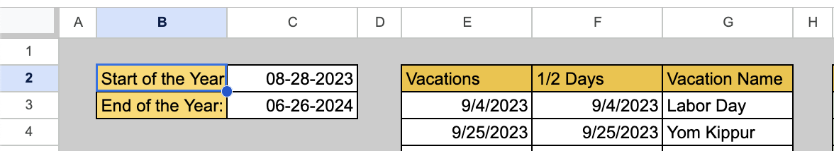
Click on the “Variables” page. Select a cell and label it “Start of the Year.” Record the start date (Month-day-year) in the right adjacent cell. Go down a row and do the same thing for the “End of the Year.”
IMPORTANT NOTE: I am using cells C3 and C3 for my start and end dates. These cells will be represented in the function below.You will have to adjust the function in the next step if you use different cells.
Skip a column on the right and record the following three headings:
Vacations | ½ days | Vacation Name
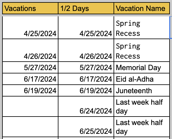
Fill out the “Vacations” chart. Every vacation day needs an entry. If Spring break is a week long it will require five represented days. Half days only get a date in the “Half day column.” Regular days off will have a date in both the “Vacations” column and the “½ day” column.
Building Your List of Dates
Now navigate to your “Instructional Days” sheet. Add a heading in cell A1 named “Dates.” I am going to add an advanced function in cell A2 that will use the start and end dates on the “variables” page to build a list of dates. The beauty of this is I can change those variables next year and the list will update! I will paste the function below and then explain what it does. Full disclosure: I will use the ChatGPT AI to break down the function and then I will edit the AI response (I did need quite a bit of editing), because it is a time saver.
Function in A1: =ArrayFormula(TO_DATE(row(indirect("C"&Variables!C2):indirect("C"&Variables!C3))))
1. indirect("C"&Variables!C2):indirect("C"&Variables!C3): are constructing cell references. They take the values in C2 and C3 from the "Variables" sheet and turns them into cell references, so if C2 contains “08-31-2023” and C3 contains “9-26-2024”, these expressions would allow you to evaluate the cells respectively. The “INDIRECT” part will keep these values dynamic. I can change the dates easily!
2. row(...): then generates an array of numbers starting from the row number of the first cell reference (C1) to the row number of the second cell reference (C10). If your two cells referenced 1 and 10, it would create an array of 10 rows, from 1 to 10. In our example, it is making a row for each date.
3. ArrayFormula(...): This function is used to apply a formula to an entire range, turning a single-cell operation into an array operation. This allows us to create a vertical list of dates that will continue until the “End Date” is reached!
4. TO_DATE(...): This forces the Sheet to use our variables as dates. It will convert a number into the corresponding date. Without this, a sheet will see a string of numbers and assume they are just numbers. We are telling the sheet that this array contains dates and that the sheet should treat them in this way.
Viola! I have a list of dates now that span the gap between my start and end dates. Magic. Now Let’s make the dates useful.
Setting the Days of the Week
We need to take that long list of dates and add context. Important information includes what days do those dates represent? Which ones are the weekend? Which ones are holidays? Sadly, you can’t have a sheet automatically distinguish a Monday from a Saturday. There is a trick, though. A function called WEEKDAY will convert a date into a numerical representation of the weekday. The sheet considers Sunday the start of the week and will represent it as number “1.” Monday will be “2” and Saturday is, you guessed it, “7.” Once we have this we can build an IF/THEN statement that will convert the numbers into week day names. Let’s start.
Select B1 on the “Instructional Sheet” and label the column “NoW” (Short for Number of weekday, but make it what you want!) In B2 we are going to add an ARRAYFORMULA. An arrayformula takes a function and applies it to a range of cells. This is super useful and cuts back on all those copy and pasted functions. I will follow the function with an explanation (using edited assistance from ChatGPT.)
Paste the following function in B2: =ARRAYFORMULA(WEEKDAY(A2:A307))
1. WEEKDAY(A2:A307): This part of the formula calculates the day of the week for each date in the range D4 to D307. It returns a number, where 1 represents Sunday, 2 represents Monday, and so on up to 7 for Saturday.
2. ARRAYFORMULA(): This is a Google Sheets function that allows you to apply a function to a range of cells and get an array of results. In this case, it's used to apply the WEEKDAY function to the entire range of dates, so you get a list of weekday numbers corresponding to the dates in A2 to A307. A2 is the first date, and A 307 is the last.
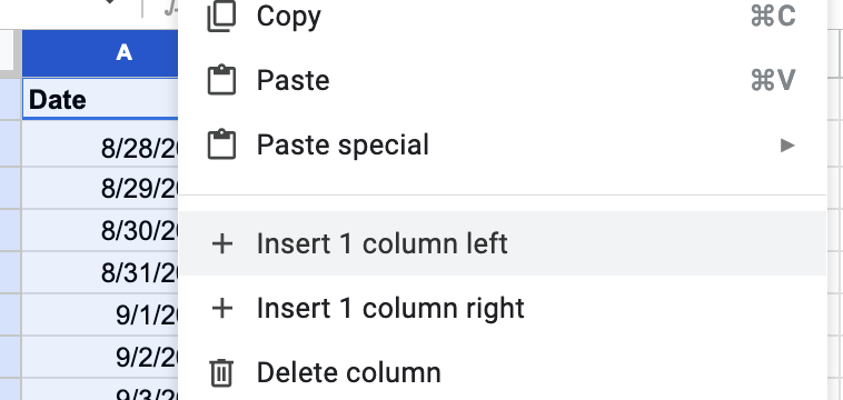
Great! Now you have a nice list that we can reference. Let's build an If/then statement that will identify those numbers. Click the heading letter at the top of column A and click the down point arrow on the right of the box. Select “Add 1 column to the left.” Label this new column “DoW.” We are going to build a statement that checks the Number of the Week column and returns a text value. This will be a nested IF/Then/Else statement in an ARRAYFORMULA.
Start by setting your function as an Array. You begin with “=ARRAYFORMULA” when setting up an array. Then add a parentheses and your first IF statement:
=ARRAYFORMULA( IF(
Our first statement is going to check for blanks and return no value. This is a handy trick that I use everywhere that I have a nested IF/THEN in an array. It prevents errors when the end of the list is reached and there are no values to check against. The Arrayformula function allows me to use a range, in this case C2:C. Function statements are surrounded by parentheses and the function components are separated by commas inside the parens.
IF(logical_expression, value_if_true, else)
I am looking for blank values (IF( C2:C="") which will return nothing (IF( C2:C="",, ). Finally, I have my “else” statement which starts my first nested IF statement.
=ARRAYFORMULA( IF( C2:C="",, IF(
The next statement starts identifying the numbers of the week in column C. All text values need to be surrounded by quotes, eg: “Monday”. Then continue with the next else statement until all seven days are represented.
=ARRAYFORMULA(If(C2:C="",,IF( C2:C=2,"Monday", IF(
Congratulations! You’ve set up your dates and identified the days of the week! Now lets determine which of those days have class.
Setting up Instructional Days
Create two columns to the left of the “DoW” column. Label these AM and PM. Let's start by indicating that our function in A1 (Column AM) will be an array and set the function to ignore blanks. Then start your nested IF/THEN/ELSE.
=ARRAYFORMULA( IF( C2:C="",, IF(
Next create your IF/Then/Else Statement to identify weekends. Write your statement for Sunday, too.
=ARRAYFORMULA( IF( C2:C="",, IF( C2:C="Saturday", "Weekend", IF(
Once the weekends are identified, we are going to exclude the holidays and conference days as “Not Instructional.” This is going to use a function called MATCH to compare the dates with our vacations list. We are going to nest this function inside a IF/THEN statement. This will compare the dates in column D with the vacation dates on our variables sheet. If a match is found, it will return “Not Instructional, else it will return “Instructional.”
IF( (MATCH( D2:D,Variables!E3:E,0)),"Not Instructional","Instructional")))))
Did you notice something went wrong? This is because values that did not return a match (the date wasn’t on the vacation list) came back as an error. Lets add a function called IFERROR that will have the match ignore these unmatched dates. We’ll add IFERROR before the MATCH parens and include the IFERROR instructions after the parens.
IF( IFERROR( MATCH( D2:D,Variables!E3:E,0))>0, "Not Instructional","Instructional")))))
Excellent! Now do this same thing for the PM column (col. B) but reference the Half Day column on the variables sheet.
Next we will make the sheet connect to lessons and allow you to change the number of days that each lesson will take to complete, allowing the dates to cascade and correct.
Extension activity: Try to figure out how to change the color of the rows based on whether Column A says “Instructional”, “Not Instructional” or Weekend. This will be a custom formula using conditional formatting.
No comments:
Post a Comment